LibreOffice Calc: Filter Pivot Table by Year
Originally Posted 7/2/25
Background Info
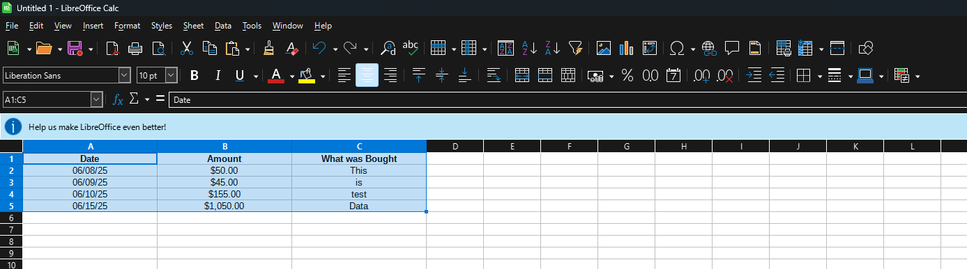
So, I keep a spreadsheet with all of my spending in it, and at the end of the year I like to make a pivot table to see where my money has gone. One thing I like is to be able to filter based on Year. I have a date column in my table, so the data is there. However, I find the pivot table functionality in LibreOffice extremely unintuitive. When I make the Pivot Table, I can choose to have my "Date" column as a filter, but then it lists every single date that's been entered, without the ability to sort by Months or Years. So, if I had to use it this way, I'd have to unselect every single unique date I've ever entered. This is, unappealing.
In Microsoft Excel, you could just drag the date option into one of the pivot table areas (I forget exactly which at this point) and it'll split into Month, Quarter, and Year. Not in LibreOffice Calc. Every time I want to do this, I have to Google how, because I just forget every time because it's just not how I'd think of it. So I wanted to make this post so next time, I can just check my own notes basically (and, of course, in case it helps anyone else).
A quick aside, I do plan on making another post at some point in the future about LibreOffice in general (it's an alternative to Microsoft Office), however I've not gotten around to it yet.
How to Filter by Year in a Pivot Table in LibreOffice Calc
- Select all of the data you'd like to include in a pivot table
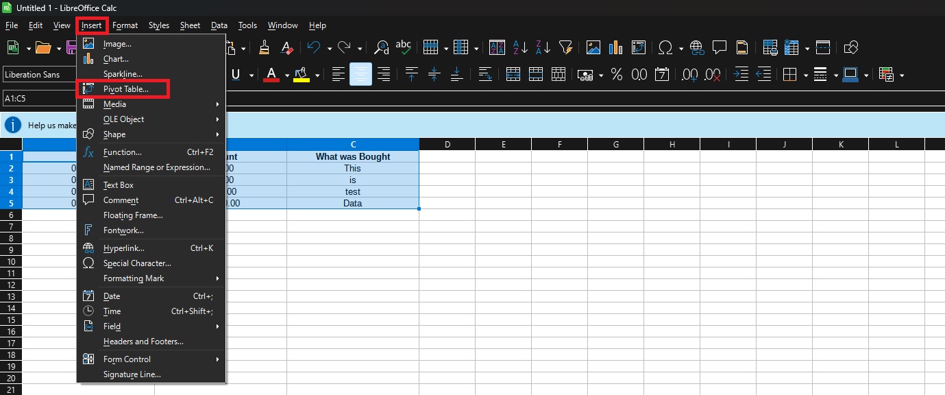
- Click "Insert" -> "Pivot Table"
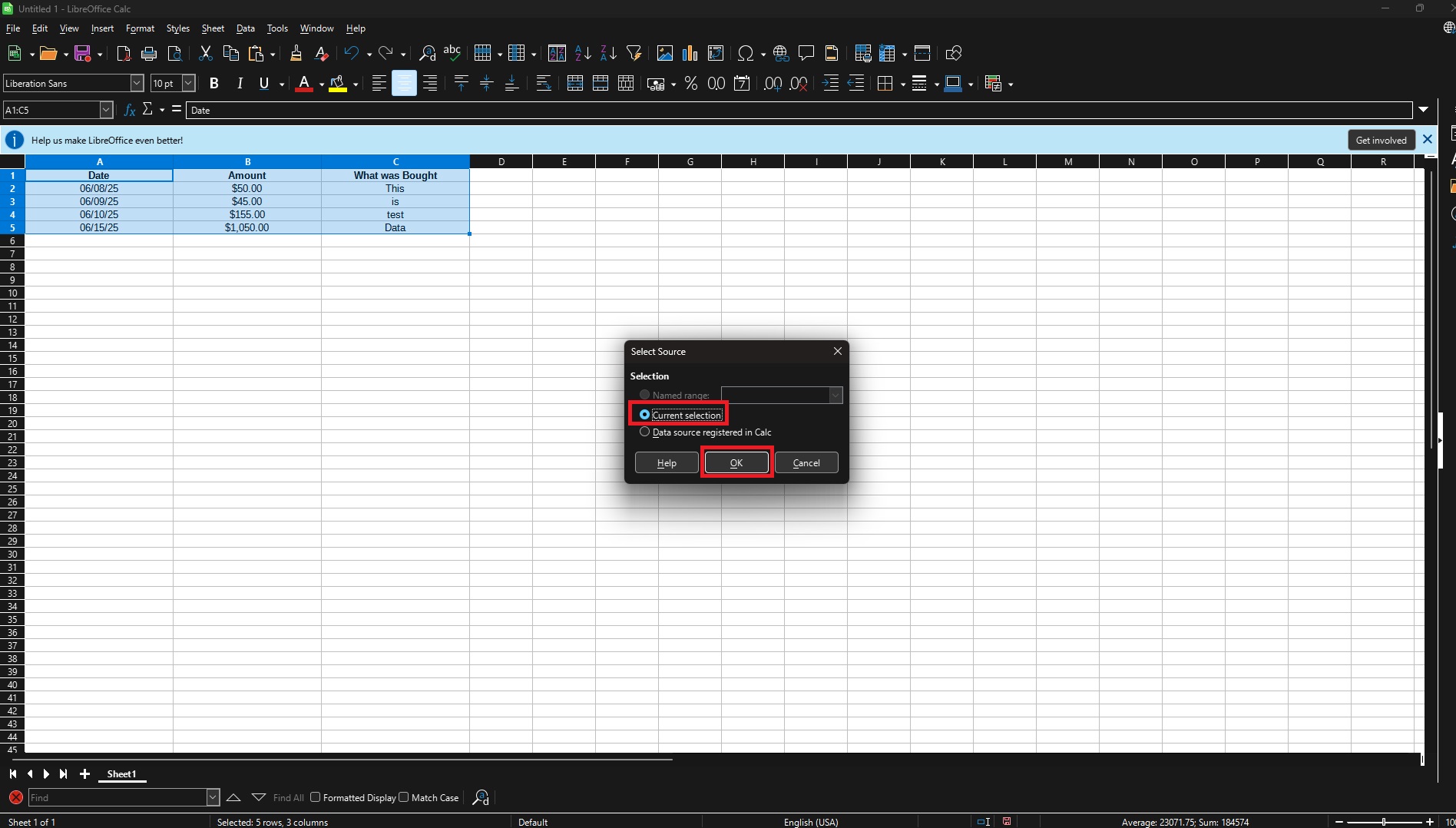
- Select "OK" with "Current Selection" selected
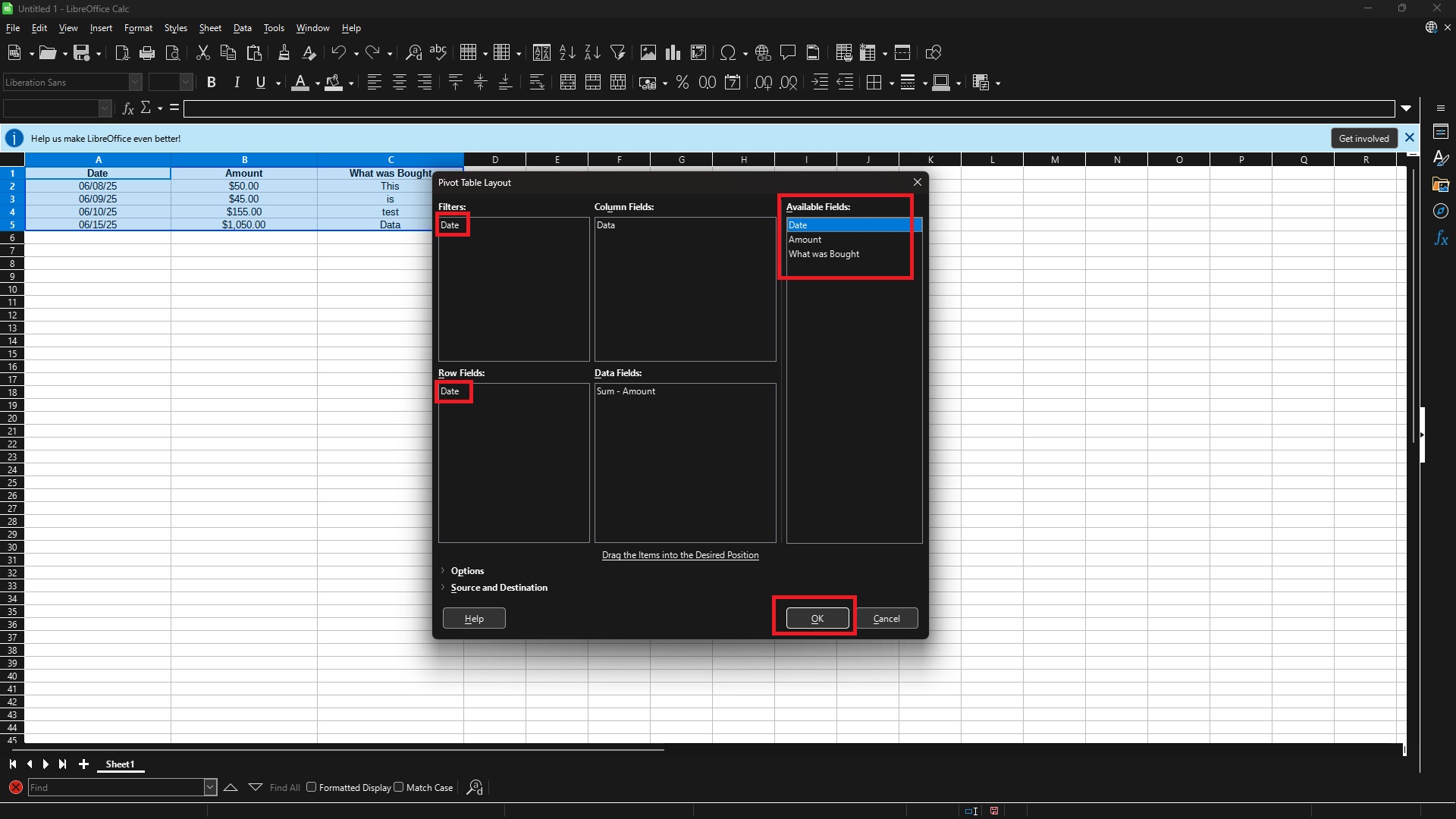
- Put "Fields" where you want them, and press "OK". Make sure the "Date" field (Or whatever you call your column with the date in it) is also in the "Row Fields" section
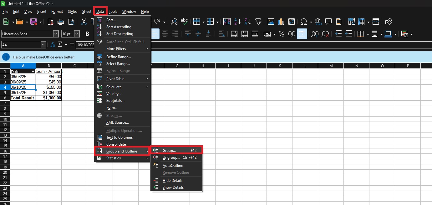
- Select anywhere in the "Date" column, then go to "Data" -> "Group and Outline" -> "Group"
- Under "Group By", select all that you would like (In my case, Months and Years), and press "OK"
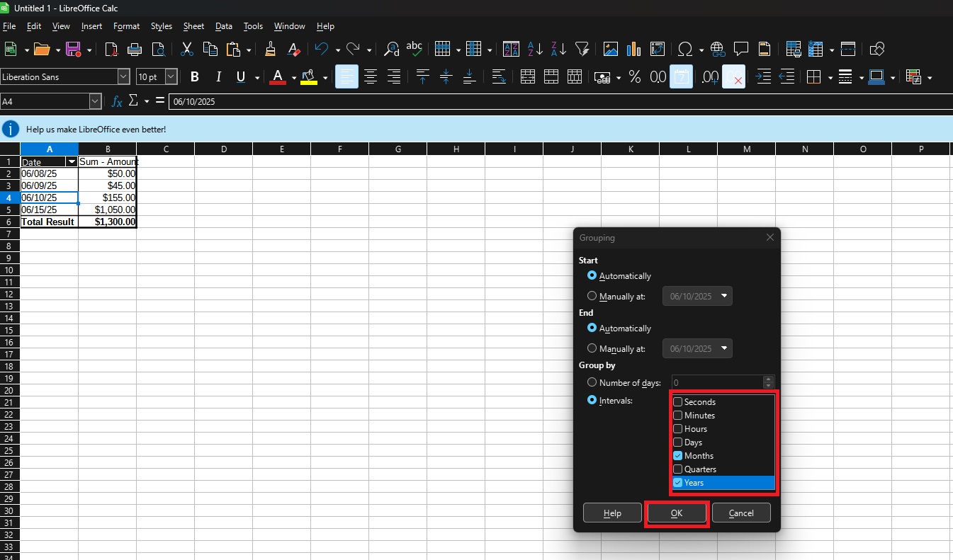
And that's it! You should be able to now filter by Year and Month (if you chose the settings I did). If you right click somewhere in the pivot table, and click "Properties", it'll bring back up the Pivot Table Layout options, and you should now have a "Years" option in the "Row Fields" you can drag up to the "Filters" Section, or leave it as is.
Wrap Up
As always, if you have any issues or suggestions, feel free to let me know!